PSIN 谣言检测——《Divide-and-Conquer: Post-User Interaction Network for Fake News Detection on Social Media》( 四 )
我们根据用户的行为构建了一个用户发布图 。如 Figure 6 所示,我们假设给定帖子的传播者可以表达其产生的社会效应模式,而用户传播的帖子描述了用户的特征 。基于此假设,我们计算了 bipartite user-post graph 的邻接矩阵 $\widehat{\mathrm{A}}^{U P} \in \mathbb{R}^{N \times M}$ 为:
$\widehat{\mathrm{A}}^{U P}=\mathrm{A}^{U P}\left(\sum_{d=1}^{d_{\max }}\left(\mathrm{A}^{P}\right)^{d}\right)$
其中,$\mathrm{A}^{U P} \in \mathbb{R}^{N \times M}$ 为 is-author graph $G^{UP}$ 的邻接矩阵,$\mathrm{A}^{P}$ 是上述增强图的邻接矩阵 。为了在 user-post graph 中使用 GNN,我们首先使用两个投影矩阵将它们的表示投影到一个统一的空间中:
$\mathbf{H}^{P}=\mathbf{W}^{P} \widehat{\mathbf{P}}, \mathbf{H}^{U}=\mathbf{W}^{U} \widehat{\mathbf{U}}$
然后,我们将该图视为齐次图,得到 $\mathbf{H}= Concat \left(\mathrm{H}^{P}, \mathrm{H}^{U}\right)$ 。邻接矩阵的定义为:
$\tilde{A}=\left[\begin{array}{cc}\mathrm{A}^{U P^{T}} & 0 \\0 & \mathrm{~A}^{U P}\end{array}\right]$
我们使用标准的 GATv2 来表示节点,每个层的更新规则是:
$\mathrm{H}^{\prime}=\mathrm{GATv} 2(\mathrm{H}, \widetilde{\mathrm{A}})+\mathrm{H} \text {. }$
我们在 post-user interaction layers 之后得到 $\widetilde{\mathbf{H}}=\left\{\widetilde{\mathbf{h}}_{1}^{P}, \widetilde{\mathbf{h}}_{2}^{P}, \ldots, \widetilde{\mathbf{h}}_{M}^{P}, \widetilde{\mathbf{h}}_{1}^{U}, \widetilde{\mathbf{h}}_{2}^{U}, \ldots, \widetilde{\mathbf{h}}_{N}^{U}\right\}$。然后我们获得帖子和用户的最终表示为 $\mathbf{P}^{\prime}=\left\{\mathbf{h}_{1}^{P^{\prime}}, \mathbf{h}_{2}^{P^{\prime}}, \ldots, \mathbf{h}_{M}^{P^{\prime}}\right\}$,$\mathbf{U}^{\prime}=\left\{\mathbf{h}_{1}^{U^{\prime}}, \mathbf{h}_{2}^{U^{\prime}}, \ldots, \mathbf{h}_{N}^{U^{\prime}}\right\}$,其中,$\mathbf{h}_{i}^{P^{\prime}}=\operatorname{Concat}\left(\widehat{\mathbf{h}}_{i}^{P}, \widetilde{\mathbf{h}}_{i}^{P}\right)$ 和 $\mathbf{h}_{i}^{U^{\prime }}=\operatorname{Concat}\left(\widehat{\mathbf{h}}_{i}^{U}, \widetilde{\mathbf{h}}_{i}^{U}\right) $ 。
4.5 Aggregation给定帖子和用户的表示:$\mathrm{P}^{\prime} \in \mathbb{R}^{M \times d}, \mathbf{U}^{\prime} \in \mathbb{R}^{N \times d}$,我们采用三个全局注意层将它们分别转换为两个固定大小的向量 。全局注意层的表述为:
$\mathbf{r}=\sum_{k=1}^{K} \operatorname{Softmax}\left(f\left(\mathbf{h}_{k}\right)\right) \odot \mathbf{h}_{k}$
其中,$f: \mathbb{R}^{d} \rightarrow \mathbb{R}$ 是一个两层 MLP 。最后,我们得到两个合并向量 $\mathbf{p}$,$\mathbf{u} $,并将它们连接起来,得到第 $i$ 个新闻事件的最终表示为 $\mathrm{z}=\operatorname{Concat}(\mathbf{p}, \mathbf{u})$ 。
4.6 Topic-agnostic Fake News Classification
文章插图
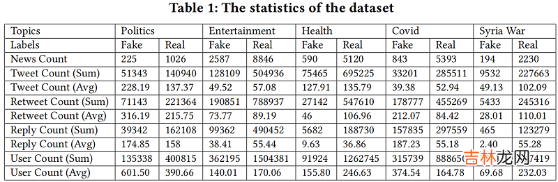
如 Table 1 所示,不同主题之间的传播特征差异很大,我们提出了一个辅助 adversarial module 和 a veracity classifier 来学习类判别和域不变节点表示 。总体目标如下:
$\mathcal{L}\left(\mathrm{Z}, \mathrm{Y}^{V}, \mathrm{Y}^{C}\right)=\mathcal{L}_{V}\left(\mathrm{Z}, \mathrm{Y}^{V}\right)+\gamma \mathcal{L}_{C}\left(\mathrm{Z}, \mathrm{Y}^{C}\right)$
其中,$\gamma$ 是平衡参数 。$\mathcal{L}_{V}$ 和 $\mathcal{L}_{C}$ 分别表示准确性分类器损失和主题分类器损失 。$Z$ 是整个数据集提取的特征矩阵,$\mathrm{Y}^{V}$ 是准确性标签,$\mathrm{Y}^{C}$ 是主题标签 。具体介绍如下:
4.6.1 Veracity Classifier Loss准确性分类器损失 $\mathcal{L}_{V}\left(\mathrm{Z}, \mathrm{Y}^{V}\right)$ 是为了最小化准确性分类的交叉熵损失:
$\mathcal{L}_{V}\left(\mathrm{Z}, \mathrm{Y}^{V}\right)=-\frac{1}{N_{t}} \sum_{i=1}^{N_{t}} y_{i}^{V} \log \left(f_{V}\left(\mathbf{z}_{i}\right)\right)$
经验总结扩展阅读


- PLAN 谣言检测——《Interpretable Rumor Detection in Microblogs by Attending to User Interactions》
- 谣言检测——《Debunking Rumors on Twitter with Tree Transformer》
- 如何检测手机
- 水质检测笔多少为正常
- 翅尖有毒是谣言吗
- 核酸检测阳性怎么办
- 自身 如何在linux下检测IP冲突
- 华为watch3pro支持血糖检测吗_华为watch3pro有测血糖功能吗
- 东莞机动车检测站周末上班吗
- Notebook交互式完成目标检测任务